Investigating the Babyface MIDI protocol
Contents
Introduction
Recently, I’ve been working on reverse engineering and documenting the MIDI SysEx protocol used to control the RME Babyface Pro audio interface, hoping to get an idea of what would be needed to add support for it to oscmix. At the very least, this documentation will enable others to write their own software to utilize the full potential of the device on Linux or other free operating systems, instead of being constrained to the features available through the physical controls.
I’m particularly interested in the EQ functionality of the device, since this is the main feature that is missing from the alsa mixer controls on Linux.
First some background: RME audio interfaces can run in two different modes: driver-based and class-compliant. Typically, on Windows and macOS, the driver mode is used with RME’s drivers, alongside TotalMix FX, a powerful control/mixer application. Class-compliant mode, on the other hand, uses the standard USB audio 2 device class, and works on any operating system that supports this. However, in class-compliant mode, there is no control/mixer software available. There is hope though, since the TotalMix FX app for iPad operates with the device in class-compliant mode, and provides nearly the full functionality of the driver-based desktop version.
There are a few obstacles with getting started: I don’t have an iPad, it doesn’t seem possible to inspect outgoing MIDI traffic in iOS, and I don’t actually have a Babyface Pro.
After asking some friends and family, I managed to borrow an iPad for a few weeks to experiment with, so this didn’t end up being an issue.
Using an intermediary device to inspect MIDI traffic
It turns out that it’s fairly easy to impersonate a USB MIDI device and inspect traffic by using a Raspberry Pi, or any Linux system with a UDC (USB device controller), connected between the iPad and the audio interface. All we need to do is configure Linux on the RPi as a USB audio gadget with the appropriate device and MIDI port names.
modprobe usb_f_midi

udc=1000480000.usb
product='Babyface Pro (XXXXXXXX)'
numports=2

cd /sys/kernel/config/usb_gadget
mkdir g1
cd g1
mkdir strings/0x409
echo "$product" > strings/0x409/product
# choose a unique serial number
echo "$product:$numports" | cksum | awk '{printf "%.15d", $1}' > strings/0x409/serialnumber

# add the midi function
mkdir functions/midi.0
echo "$numports" > functions/midi.0/in_ports
echo "$numports" > functions/midi.0/out_ports

mkdir configs/c.1
ln -s functions/midi.0 configs/c.1/

echo "$udc" > UDC
Now, we can dump MIDI traffic that the iPad app is sending with
aseqdump -p f_midi:1, and we can use aconnect to establish
bidirectional connections between the gadget port and the real
device port… if only we had access to the device.
Tunneling MIDI over SSH
It seems that the Babyface Pro is one of the more popular RME audio interfaces used by Linux users. There is decent support for it in recent upstream Linux kernels, and it was requested by several people in the oscmix issue tracker. However, my early investigation into the Babyface Pro indicated that it worked quite differently from other RME devices. The sysex packet structure and overall protocol that I had become familiar with from my investigation with my UCX II did not seem to apply.
However, one day I was talking to someone on IRC with the device and I had the idea to simply tunnel the MIDI traffic to and from my RPi to their device. I’m not sure if there is some common way to send MIDI over the internet, but I ended up writing a small tool called alsaseqio that simply reads and/or writes a MIDI bytestream from stdin/stdout to an alsa sequencer port. I’m quite happy with how it turned out and I think it could be quite a useful tool in general. I’m using it in place of platform-specific MIDI code in oscmix.
# on remote system with device
alsaseqio -p Babyface:1 ssh user@mypi alsaseqio
This reads and writes from the Babyface MIDI port to a new alsa sequencer port on my RPi. Now, all I need to do is connect the alsaseqio port to the MIDI gadget port. I could have made the RPi instance of alsaseqio connect directly to this port, but I figured having a separate port would be easier if I needed to bring the gadget down and back up during my investigation without bothering the device owner.
aconnect f_midi:1 alsaseqio
It turns this did come back to bite me. After an hour or so of being
confused as to why it wasn’t working, I remembered that aconnect
only establishes a unidirectional connection. I also needed to make
the reverse connection.
aconnect alsaseqio f_midi:1
Now we’re in business! I can fiddle with controls on the iPad, and see what gets sent over MIDI. I can also ask the device owner to interact with it on his end and see what gets sent back.
Decoding the MIDI SysEx messages
My initial suspicions were correct; the protocol used by the Babyface is quite different from the UCX II. The tools I had developed to analyze it did not work. However, there were some similarities in the packet format and overall structure that made early progress much quicker. The sysex messages had the same form:
      Manufacturer ID
      |
   /------\
F0 00 20 0D 10 <subid> <payload> F7
|           |                    |
SysEx start Device ID            SysEx end
The payload of a sequence of 32-bit integers encoded as five 7-bit bytes each (sysex message bytes cannot have their high bit set) with little-endian byte order. The sub ID is a single byte indicating the message type.
From here, it wasn’t too difficult to notice that the app sent messages with sub ID 6 to control the equalizer. Let’s try changing the EQ settings in the app for channel 1 and record what we get.
# cycle band 2 (peak) through frequencies [100, 300, 1000, 3000, 10000] at 20 dB and Q=1
80000000 00000000 00000000 00000000 00000000 F008CF60 07F78A41 F0536637 07ACF1C6 00000000 00000000 00000000 00000000 082611DB 04000000 00000000
80000000 00000000 00000000 00000000 00000000 F01C6998 07E6B9DB F0F26A8A 07108EA4 00000000 00000000 00000000 00000000 0871BBA4 04000000 00000000
80000000 00000000 00000000 00000000 00000000 F075546B 07AD007F F2DB0027 05420928 00000000 00000000 00000000 00000000 09757DC3 04000000 00000000
80000000 00000000 00000000 00000000 00000000 F213AED2 0711FD39 F6DBA1D6 01E5322B 00000000 00000000 00000000 00000000 0C2F0C7D 04000000 00000000
80000000 00000000 00000000 00000000 00000000 FC870372 056AC7A8 FE9592E6 FD784E9D 00000000 00000000 00000000 00000000 139F7D8F 04000000 00000000
# set the gain of band 1 (shelf) to -15 dB and 100 Hz, and band 2 to 10 dB
80000000 F029B117 07D721C0 F0117B95 07EEAA22 FCEA3CDD 03EB681F FE02F2F8 FFAED24D 00000000 00000000 00000000 00000000 0C56C113 04000000 00000000
Analyzing the EQ messages
Each time the EQ settings change, we see a message with sub ID 6 and a payload consisting of 16 32-bit integers. It’s pretty clear that indices 5-8 correspond to band 2, and indices 1-4 correspond to band 1. Following this pattern, indices 9-12 likely correspond to band 3. We also see that index 14 changes regardless of the band we changed.
Unfortunately, there doesn’t seem to be much structure to the integers themselves. On the UCX II, the EQ was controlled parametrically. There was an address for band 1 cut-off, band 1 gain, band 1 Q, etc. When the band 1 cut-off was changed to 3000, 3000 was written to a particular address. This made it easy to see what was going on and write software to interact with these controls. Here, all four integers corresponding to the band change at once with no discernable pattern.
This is a strong indication that these integers represent digital filter coefficients used to implement the EQ. This is also supported by the fact that the integers change all at once when the device sample rate is changed, since the cut-off frequency in radians/second depends on the sample rate.
A common technique for implementing digital EQ is to use digital biquadratic filters. These are filters whose transfer function is the ratio of two quadratic functions.
If we normalize both the numerator and denominator, and calculate an overall gain coefficient, we end up with
Let’s redefine , , and .
Two of these filters in series would look like
This is starting to resemble what we are seeing in the sysex messages. Four coefficients per band, plus one overall gain coefficient.
The excellent Audio EQ Cookbook by Robert Bristow-Johnson gives formulas for coefficients for various filter types from their parameters. Trying out the peaking filter formulas with typical parameter values, we get coefficients around -2 to 2.
import numpy as np
import pandas as pd

def peak(gain, freq, Q, samplerate):
  A = 10**(gain/40)
  omega_0 = freq/samplerate*2*np.pi
  alpha = np.sin(omega_0) / (2*Q)
  a0 = 1 + alpha/A
  a1 = -2*np.cos(omega_0)
  a2 = 1 - alpha/A
  b0 = 1 + alpha*A
  b1 = a1
  b2 = 1 - alpha*A
  return pd.Series({
      'a1': a1 / a0,
      'a2': a2 / a0,
      'b1': b1 / b0,
      'b2': b2 / b0,
      'c': b0 / a0,
  })

# 20 dB gain, peak at 1000 Hz, Q of 1, 48 kHz sample rate
peak(20, 1000, 1, 48000)
| a1 | -1.942794 |
|---|---|
| a2 | 0.959559 |
| b1 | -1.643669 |
| b2 | 0.657852 |
| c | 1.181986 |
Looking back at the data we’ve gathered, we see that some of the
coefficients begin with 0 and some begin with F. Let’s put this
data into a table and try interpreting them as two’s complement
signed integers.
import pandas as pd

df = pd.DataFrame([
    [0x80000000, 0x00000000, 0x00000000, 0x00000000, 0x00000000, 0xF008CF60, 0x07F78A41, 0xF0536637, 0x07ACF1C6, 0x00000000, 0x00000000, 0x00000000, 0x00000000, 0x082611DB, 0x04000000, 0x00000000],
    [0x80000000, 0x00000000, 0x00000000, 0x00000000, 0x00000000, 0xF01C6998, 0x07E6B9DB, 0xF0F26A8A, 0x07108EA4, 0x00000000, 0x00000000, 0x00000000, 0x00000000, 0x0871BBA4, 0x04000000, 0x00000000],
    [0x80000000, 0x00000000, 0x00000000, 0x00000000, 0x00000000, 0xF075546B, 0x07AD007F, 0xF2DB0027, 0x05420928, 0x00000000, 0x00000000, 0x00000000, 0x00000000, 0x09757DC3, 0x04000000, 0x00000000],
    [0x80000000, 0x00000000, 0x00000000, 0x00000000, 0x00000000, 0xF213AED2, 0x0711FD39, 0xF6DBA1D6, 0x01E5322B, 0x00000000, 0x00000000, 0x00000000, 0x00000000, 0x0C2F0C7D, 0x04000000, 0x00000000],
    [0x80000000, 0x00000000, 0x00000000, 0x00000000, 0x00000000, 0xFC870372, 0x056AC7A8, 0xFE9592E6, 0xFD784E9D, 0x00000000, 0x00000000, 0x00000000, 0x00000000, 0x139F7D8F, 0x04000000, 0x00000000],
    [0x80000000, 0xF029B117, 0x07D721C0, 0xF0117B95, 0x07EEAA22, 0xFCEA3CDD, 0x03EB681F, 0xFE02F2F8, 0xFFAED24D, 0x00000000, 0x00000000, 0x00000000, 0x00000000, 0x0C56C113, 0x04000000, 0x00000000]
])
df = df.iloc[:, 1:14].astype(np.int32)
df.style.format('{:X}')
| 1 | 2 | 3 | 4 | 5 | 6 | 7 | 8 | 9 | 10 | 11 | 12 | 13 |
|---|---|---|---|---|---|---|---|---|---|---|---|---|
| 0 | 0 | 0 | 0 | -FF730A0 | 7F78A41 | -FAC99C9 | 7ACF1C6 | 0 | 0 | 0 | 0 | 82611DB |
| 0 | 0 | 0 | 0 | -FE39668 | 7E6B9DB | -F0D9576 | 7108EA4 | 0 | 0 | 0 | 0 | 871BBA4 |
| 0 | 0 | 0 | 0 | -F8AAB95 | 7AD007F | -D24FFD9 | 5420928 | 0 | 0 | 0 | 0 | 9757DC3 |
| 0 | 0 | 0 | 0 | -DEC512E | 711FD39 | -9245E2A | 1E5322B | 0 | 0 | 0 | 0 | C2F0C7D |
| 0 | 0 | 0 | 0 | -378FC8E | 56AC7A8 | -16A6D1A | -287B163 | 0 | 0 | 0 | 0 | 139F7D8F |
| -FD64EE9 | 7D721C0 | -FEE846B | 7EEAA22 | -315C323 | 3EB681F | -1FD0D08 | -512DB3 | 0 | 0 | 0 | 0 | C56C113 |
The absolute value of most of these numbers fall in the range
[-2*0x8000000, 2*0x8000000], so let’s rescale them to be in the
expected range.
df = df / 0x8000000
df
| 1 | 2 | 3 | 4 | 5 | 6 | 7 | 8 | 9 | 10 | 11 | 12 | 13 |
|---|---|---|---|---|---|---|---|---|---|---|---|---|
| 0.000000 | 0.000000 | 0.000000 | 0.000000 | -1.995698 | 0.995869 | -1.959278 | 0.959446 | 0.0 | 0.0 | 0.0 | 0.0 | 1.018589 |
| 0.000000 | 0.000000 | 0.000000 | 0.000000 | -1.986127 | 0.987659 | -1.881633 | 0.883085 | 0.0 | 0.0 | 0.0 | 0.0 | 1.055534 |
| 0.000000 | 0.000000 | 0.000000 | 0.000000 | -1.942710 | 0.959474 | -1.643066 | 0.657244 | 0.0 | 0.0 | 0.0 | 0.0 | 1.182369 |
| 0.000000 | 0.000000 | 0.000000 | 0.000000 | -1.740389 | 0.883784 | -1.142758 | 0.236912 | 0.0 | 0.0 | 0.0 | 0.0 | 1.522973 |
| 0.000000 | 0.000000 | 0.000000 | 0.000000 | -0.434075 | 0.677139 | -0.176966 | -0.316256 | 0.0 | 0.0 | 0.0 | 0.0 | 2.452876 |
| -1.979643 | 0.980045 | -1.991464 | 0.991535 | -0.385626 | 0.489945 | -0.248560 | -0.039638 | 0.0 | 0.0 | 0.0 | 0.0 | 1.542360 |
This seems very promising. Row 3 almost exactly matches the coefficients that we calculated earlier. Let’s plot the frequency response and see if we get anything sensible.
import control as ct
from matplotlib import pyplot as plt
plt.rcParams['figure.figsize'] = (10, 6)

def band(val):
  return ct.tf([1, val[2], val[3]], [1, val[0], val[1]], 1/48000)
def eq(row):
  val = row.values
  H = val[12]*band(val[0:4])*band(val[4:8])*band(val[8:12])
  H.name = str(row.name)
  return H
fig, ax = plt.subplots()
for H in df.apply(eq, axis=1):
  ct.bode_plot(H, Hz=True, dB=True, plot_phase=False, omega=(20*2*np.pi, 48000*np.pi), ax=ax)

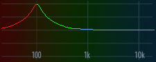
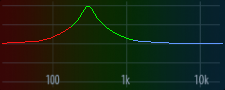
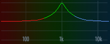
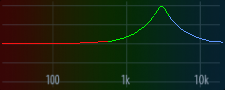
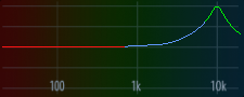
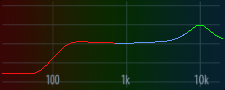
This is exactly what we were hoping to see! The peak moves higher as we adjust the cut-off from 100 to 300, 1000, 3000, and 10000 (roughly equally spaced in ), and then shrinks to 10 dB while the shelf appears at -15 dB and 80 Hz.
Frequency warping
Even though our calculated coefficients match almost exactly at 1000 Hz, as the peak frequency gets closer to the Nyquist rate (half the sample rate) they start to drift, and the peak of the filter with our calculated coefficients starts to get compressed horizontally.
f0 = 18000
df = pd.DataFrame([
    pd.Series({'a1': 0x08C17449, 'a2': 0x0461E521, 'b1': 0x02E28F51, 'b2': 0xFC147B3A, 'c': 0x184778F1}).astype(np.int32) / 0x8000000,
    peak(20, f0, 1, 48000),
], index=['totalmix', 'calculated'])

fig, ax = plt.subplots()
kw = {'Hz': True, 'dB': True, 'plot_phase': False, 'omega': (4800*2*np.pi, 48000*np.pi), 'ax': ax}
for H in df.apply(lambda s: ct.tf(s.c*np.array([1, s.b1, s.b2]), [1, s.a1, s.a2], 1/48000, name=s.name), axis=1):
  ct.bode_plot(H, **kw)

# prototype analog filter
Omega_0 = f0*2*np.pi
H = ct.tf([1, 10**(20/40)*Omega_0, Omega_0**2], [1, 10**(-20/40)*Omega_0, Omega_0**2], name='analog')
ct.bode_plot(H, **kw)

df
| a1 | a2 | b1 | b2 | c | |
|---|---|---|---|---|---|
| totalmix | 1.09446 | 0.547800 | 0.360625 | -0.489999 | 3.034899 |
| calculated | 1.27200 | 0.798879 | 0.667701 | -0.055728 | 1.905044 |

What’s happening here is called frequency warping and is an artifact of the bilinear transform used to digitize the analog prototype filter. This happens because we are mapping the infinite frequency axis in the s-domain onto the unit circle in the Z-domain.
The bilinear transform allows us to ensure one frequency of the analog filter is mapped to a particular frequency of the resulting digital filter. The equations we used to calculate the coefficients ensure that the peak appears at the frequency we specified. However, other frequencies, (normalized so peak is at 1), get warped to as follows:
fig, ax = plt.subplots()
ax.set_aspect('equal')
ax.set_xlabel(r'digital frequency [Hz]')
ax.set_ylabel(r'analog frequency [Hz]')
ax.set_xscale('log')
ax.set_yscale('log')
omega_0 = f0/48000*2*np.pi
Omega_hat = np.logspace(-2, 2, 1000)
omega = 2*np.arctan(Omega_hat*np.tan(omega_0/2))
ax.plot(omega*48000/(2*np.pi), Omega_hat*f0)
ax.scatter(omega_0*48000/(2*np.pi), Omega_0/(2*np.pi), label=f'{f0} Hz')
ax.legend()
plt.show()

In this graph, we see an asymptote at the Nyquist rate, caused by packing an infinite range of analog frequencies into a small range of digital frequencies.
What’s TotalMix doing here to compensate for this bandwidth cramping? Stay tuned for a follow-up post where I’ll investigate several different choices for instead of and how they compare for different and .
Conclusion
In this post, I’ve focused on controlling EQ settings, but there’s a lot more I didn’t cover including the mixer, channel gain, peak/RMS meter values, physical device controls, and more. I’ve put up my notes on the oscmix wiki at Babyface Pro for anyone that’s interested.
Given the differences between the Babyface and other Fireface devices, it will take some time to think of a good way to architect oscmix to support both classes of devices, but should be possible.
This was a fun exercise in reverse engineering, MIDI, and signal processing. It was nice to refresh myself on signal processing, which was one of my favorite subjects in school, but one that I haven’t studied much since then.